Running HOS-Ocean
HOS-ocean has been developed for command-line run with an input file containing all specifications needed (name can be arbitrary but will be referred to input_HOS.dat in the following for clarity). The following commands can be executed:
Linux environment (in a terminal):
./HOS-ocean input_HOS.dat
Windows environment (using the standard command prompt
cmd):
HOS-ocean.exe input_HOS.dat
Note
All output files will be created in a directory Results that has to be created before the run by the user.
Note
For Visual Studio users, the file input_HOS.dat and the .cof file need to be placed on the same folder as the Visual Studio project.
Input file
The input file has the following form and is assumed to be named input_HOS.dat. This subsection describes in details the content of the file.
--- General info test case studied
Restart previous computation                     :: i_restart     :: 0
Choice of computed case (definition of wave)     :: i_case        :: 3
--- Geometry of the horizontal domain
Length in x-direction                            :: xlen          :: 20.0
Length in y-direction                            :: ylen          :: 20.0
--- Relaxation zones
Use of absorption/generation                     :: i_rlx         :: 0
Type of zones                                    :: i_abs         :: 1
Length 1st absorbing zone                        :: L_abs_1       :: 10.0
Length generation zone                           :: L_gene        :: 10.0
Length 2nd absorbing zone                        :: L_abs_2       :: 10.0
--- Time stuff
Duration of the simulation                       :: T_stop        :: 100.000
Sampling frequency (output)                      :: f_out         :: 20.0
Tolerance of RK scheme                           :: toler         :: 1.0e-8
Dommermuth initialisation                        :: n             :: 4
Dommermuth initialisation                        :: Ta            :: 10.0
--- Physical dimensional parameters
Gravity (in m.s-2)                               :: grav          :: 9.81
Mean water depth (real number in m)              :: depth         :: -35.
--- Current parameters
Current type (0 ; 1 or 2)                        :: i_curr        :: 0
Constant current velocity (m/s)                  :: u_0           :: 1.0
Length varying current zone 1                    :: L_curr_1      :: 10.0
Length varying current zone 2                    :: L_curr_2      :: 10.0
--- Bathymetry parameters
Definition of bottom profile used                :: i_bottom      :: 0
Choice of the method (0,1,2) for wave-bottom     :: i_method      :: 0
Total (boundary) water depth (real number in m)  :: depth_tot     :: 0.10
Minimum water depth (real number in m)           :: depth_min     :: 30.0
Bathymetry filename                              :: bathy_file    :: /bathy_new_cut.dat
Zone 1 y direction  (number of lambda)           :: L_1_y         :: 0.0
Zone 2 y direction  (number of lambda)           :: L_2_y         :: 0.0
Reflection conditions 1='yes',0='no'             :: i_sym         :: 0
--- Irregular waves (i_case=3x)
Peak period in s  (in s)                         :: Tp_real       :: 10.0
Significant wave height (in m)                   :: Hs_real       :: 4.5
JONSWAP Spectrum                                 :: gamma         :: 3.3
TMA Spectrum  (0 or 1)                           :: i_TMA         :: 0
Directionality function  (0,1,2)                 :: i_dir_JSWP    :: 1
Directionality (Dysthe)   (in radians)           :: beta          :: 1.57
Random phases generation                         :: random_phases :: 1
Name input spectrum (31,33)                      :: filename_spec :: SPEC_20181006-01_SKOREA.2D
--- Soliton's parameters (case 4x)
Carrier wave number                              :: k0            :: 5.32214
Steepness of the carrier wave                    :: eps0          :: 0.02
Initial location soliton (dim)                   :: x0            :: 60.0
--- Output files
Tecplot version                                  :: tecplot       :: 11
Output: 1-dim. ; 0-nondim.                       :: i_out_dim     :: 1
3d free surface quantities                       :: i_3d          :: 1
3d modes                                         :: i_a_3d        :: 1
2d free surface, center line                     :: i_2d          :: 0
Wave probes in domain                            :: i_prob        :: 0
Swense output 1='yes',0='no'                     :: i_sw          :: 0
--- Discretization
Number of points in x-dir.                       :: n1            :: 256
Number of points in y-dir.                       :: n2            :: 128
HOS nonlinearity order (free-surface)            :: mHOS          :: 3
HOS nonlinearity order (bottom)                  :: M_l           :: 1
Dealiasing parameters in x                       :: p1            :: 3
Dealiasing parameters in y                       :: p2            :: 3
Output points in x-dir. (i_3d=2)                 :: n1_out        :: 256
Output points in y-dir. (i_3d=2)                 :: n2_out_all    :: 1
--- Wave breaking parameters (unidirectional wave only)
Breaking model type                              :: ibrk          :: 0
Tian's breaking threshold                        :: threshold     :: 0.85
Tian's eddy viscosity                            :: alpha_eddy_vis:: 0.02
Ramp length eddy viscosity                       :: ramp_eddy     :: 0.25
Change breaking length                           :: fact_Lbr      :: 1.0
Change breaking duration                         :: fact_Tbr      :: 1.0
Cubic spline interpolant                         :: numspl        :: 5
Additional const viscosity                       :: eqv_vis       :: 0.0
--- Chalikov filter parametrization
Chalikov filter order                            :: order_filt    :: 1
Chalikov filtering strength                      :: r_filt        :: 0.25
Chalikov filtering start                      :: coeffilt_chalikov:: 0.9
--- Chalikov diffusion parametrization
Chalikov diffusion strength                      :: Cb            :: 0.01
Chalikov threshold curvature                     :: threshold_s   :: 200.0
Description of initial conditions
i_restartdescribes the possible restart of a computation that has stopped before the endi_restart=0: computation is defined only with the input file. Restart files will be created for possible use afterwards.i_restart=-1: computation is defined only with the input file. Restart files will not be created.i_restart=1: Restart from a previous computation. It should be executed in the exact same folder than the initial computation executed withi_restart=0
i_casedescribes the initial (t=0) wave conditioni_case=1: Starting from rest (useless for now)i_case=2x: Natural modes, which initial characteristics of the free surface elevation are provided in the filemodes.inp. In this file, each line describe a mode as: mode_number in x, mode_number in y (only if 3D simulation), amplitude, phasei_case=2: Progressive natural modes, velocity potential defined from free surface elevation assuming linear wave theoryi_case=21: Standing natural modesi_case=22: Progressive natural modes, velocity potential defined with another file (same format) describing its modesmodes_phi.inp
i_case=3xis used for irregular directional sea-state which characteristic is specified in the dedicated input file sectioni_case=3: initialisation from a theoretical spectrum defined as S(ω,θ)=F(ω).G(θ) with F(ω) a JONSWAP frequency spectrum and G(θ) a directional functioni_case=31: initialisation with a spectrum file extracted from WAVEWATCH III®i_case=32: initialisation from previous HOS-ocean simulationTemporal surface quantities are read from a file named
3d_ini.datThe file
3d_ini.datshould have the same structure as the classical output of the free surface information of HOS, namely3d.dat. The only difference is that it should contain only one time-step (in addition to the classical header). For this time step, you should have two columns containing for this time step the free surface elevation and the free surface velocity potential.
i_case=33: initialisation with a spectrum file containing the description of the directional spectrum S(ω,θ)i_case=34: initialisation from theoretical spectra defining two crossing sea states S1 (ω,θ)+S2 (ω,θ)
i_case=4xis used for initialisation with analytical solutions to NonLinear Schrödinger equation. The characteritics of the analytical solution is specified in the dedicated input file sectioni_case=4is used for envelope solitoni_case=40is used for the interaction of two envelope solitonsi_case=41is used for Peregrine solitoni_case=42is used for Akhmediev breatheri_case=43is used for Kuznetsov-Ma soliton
i_case=5is used for the initialisation using linear regular wavei_case=6x/7x/8x: Nonlinear regular wave from stream function theory. Each case require the presence of an external file (xxx.cof) that contains the stream function coefficients. Note that those files are generated using the CN-Stream package [Ducrozet et al., 2019]. New regular waves configurations are consequently easily accessible. In the following descriptions k stands for the wavenumber, a the wave amplitude and h the water depth.i_case=6x/7x: Finite water depth configurations used for specific applications. Some examples:i_case=60corresponds to kh=0.5 and ka=0.1i_case=61corresponds to kh=0.6725 and ka=0.1i_case=62corresponds to kh=1.0 and ka=0.1i_case=63corresponds to kh=3.0 and ka=0.1i_case=64corresponds to kh=10.0 and ka=0.1
i_case=8x: Infinite water depth configurations withka=0.x, existing cases arex=[09,1,2,3,4]. For instancei_case=82meanska=0.2
Geometry of the horizontal domain
xlenandylenare interpreted as integers and represent the number of wavelengths (i_case=4x/5/6x/7x/8x) or peak wavelengths (i_case=3x) in the domain. In the presence of relaxation zones (see next item), this is the size of the computational domain without the relaxation zones, see Fig. 4
Relaxation zones
i_rlxspecifies if relaxation zones are used (1/2/3) or not (0)i_rlx=0is the original and standard HOS configuration: no relaxation zones are used (L_abs_1=L_abs_2=L_gene=0 in Fig. 4)i_rlx=1indicates the use of generation zones together with the absorption zones defined withi_absparameter. At initial stage (t=0) the solution is zero in the central domain (between relaxation zones see Fig. 4)i_rlx=2indicates that no generation zones are used (useless for now)i_rlx=3same asi_rlx=1but at initial stage (t=0) the solution is imposed in the central domain (between relaxation zones)
i_absspecifies the type of absorptioni_abs=1: standard configuration for relaxation zones represented in Fig. 4. Two absorption zones located close to the boundaries force the solution to zero to ensure periodicity and absorb waves. Another relaxation zone ensures the generation on the left side of the domaini_abs=0: no absorption to zero. The absorption zone on the left side disappear (L_abs_1=0) and the two remaining zones ensure periodicity and wave absorption by forcing the solution toward the target solution (specified withi_case)i_abs=2: same asi_abs=1but on the right side, the absorption is not achieved by relaxation but by a pressure term added to the dynamic free surface boundary condition: parabolic dampingi_abs=3: same asi_abs=1but on the right side, the absorption is not achieved by relaxation but by a pressure term added to the dynamic free surface boundary condition: Clamond’s method
L_abs_1specifies the length of the first (left) absorbing zone (number of wavelengths), see Fig. 4L_genespecifies the length of the generation zone (number of wavelengths), see Fig. 4L_abs_2specifies the length of the second (right) absorbing zone (number of wavelengths), see Fig. 4
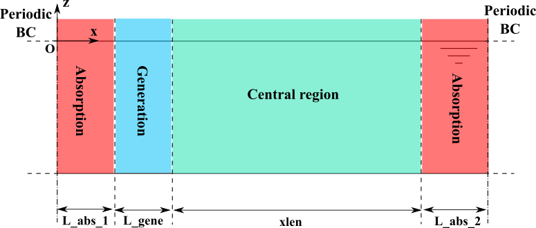
Fig. 4 Sketch of the relaxation zones arrangement
Time stuff
T_stopandf_outare defined with respect to the wave period (i_case=4x/5/6x/7x/8x) or peak period (i_case=3x)T_stopis the duration of the simulationf_outgives the output frequency of the output files described in dedicated input file section
tolergives the tolerance of the adaptative Runge-Kutta schemenandTaare the parameters of the relaxation at initial stages of computations [Dommermuth, 2000].
Physical dimensional parameters
gravdefines the gravity acceleration (in m.s-2)depthdefines the water depth (in m). A negative value stands for an infinite water depth configuration
Warning
In the case of varying bathymetry, this parameter defines the mean water depth. The bottom variations being defined with respect to this mean water depth.
Current parameters
i_currdefines the use of current (always constant over the water depth)i_curr=0: no current (standard original HOS configuration)i_curr=1: constant current in horizontal space, throughout the whole domaini_curr=2: spatially varying current, as sketched in Fig. 5
u_0: value of the current (in m/s). Positive value is along positive x-axis (following current) while negative value stands for an opposing currentL_curr_1: length of the varying current zone on the left side (number of wavelengths), see Fig. 5L_curr_2: length of the varying current zone on the right side (number of wavelengths), see Fig. 5
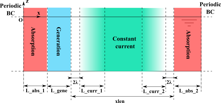
Fig. 5 Sketch of the general configuration with current
Bathymetry parameters
i_bottomdefines which bathymetry configuration is used. This covers the different test cases in [Gouin et al., 2016, Gouin et al., 2017]i_bottom=0: flat bottom (standard original HOS configuration)i_bottom=1: underwater bar configuration studied experimentally in [Dingemans, 1994]i_bottom=2: shoaling of water wavesi_bottom=4: flat bottom that can be used to test the accuracy of the wave propagation withdepth≠depth_toti_bottom=5: bottom ripplesi_bottom=6: underwater bar configuration studied experimentally in [Ohyama et al., 1995]i_bottom=7: 3D elliptical shoal studied experimentally in [Vincent and Briggs, 1989]
i_methoddefines in the case of varying bottom (i_bottom≠0) the method used to evaluate the influence of the varying bathymetry on the wave fieldi_method=0: original HOS method, no influence of the bathymetryi_method=1: same order of nonlinearity used for the expansion on the free surface (original HOS method) and the bottom variationi_method=2: different orders of nonlinearity can be used for the free surface expansion (mHOSparameter) and bottom variation (M_lparameter)
depth_totdefines the water depth (in m) in the relaxation zones used for wave generationdepth_mindefines, in the case of a file describing the bathymetry, the minimum water depth (in m) taken into account. This prevents numerical instabilities encountered for too large depth variationsbathy_file: name of the file describing the bathymetryL_1_ydefines, in the y-direction, the length of the zone where the bathymetry is gradually forced to reach the valuedepthat y=0 to ensure periodicityL_2_ydefines, in the y-direction, the length of the zone where the bathymetry is gradually forced to reach the valuedepthat y=ylen to ensure periodicityi_symindicates if reflection conditions are used in the y-direction instead of periodicity. If so (i_sym=1) the bathymetry is made symmetrical at y=ylen
Irregular waves features (i_case=3x)
Tp_realis the peak period (in s) of the irregular sea state studied (i_case=3,34)Hs_realis the significant wave height (in m) of the irregular sea state studied (i_case=3,34)gammais the JONSWAP shape parameter of the irregular sea state studied (i_case=3,34)i_TMAspecifies the use of TMA spectrum (i.e. shallow water correction of the JONSWAP spectrum) ifi_TMA=1. Usei_TMA=0for standard configurationi_dir_JSWPspecifies the type of directional spreading function G(θ) to use:i_dir_JSWP=0: the directional function is defined as G(θ) = 1/β cos²(2πθ/(4β))i_dir_JSWP=1: the directional function is the one proposed in [Hasselmann et al., 1980]: G(θ) = 1/N cos2s (θ/2) with N a normalization factor and s parameterized regarding observations in the previous referencei_dir_JSWP=2: the directional function is the wrapped-normal distribution represented as a Fourier seriesG(θ) = 1/(2π) + ∑j [1/π exp(-(j*β)2 /2) cos(j(θ-θ0 ))]
betais the value of the β parameter in previous equationsrandom_phasesspecifies the behaviour of random numbers for the choice of phases in irregular wavesi_case=3xrandom_phases=0: Random numbers are the same at every run for a given spatial discretization (i.e. a specific value ofn1andn2)random_phases=1: Random numbers are different at every runrandom_phases=-1: Random numbers are always the same (whatever the choice of discretization)random_phases>100: Use the value ofrandom_phasesas a seed value for random number generation
filename_specspecifies the name of the input wave spectrum file used wheni_case=31/33
Note
i_case=34 Since additional parameters are necessary in the case of a crossing sea state, for this specific case, the input file is slightly different and the irregular waves features has the following form (rest of the input file unchanged). As a reminder the initial wave condition is defined as S(ω,θ)=S1 (ω,θ)+S2 (ω,θ)
-- Irregular waves (i_case=3x)
Peak period in s  (in s)                         :: Tp_real       :: 15.0
Significant wave height (in m)                   :: Hs_real       :: 3.50
JONSWAP Spectrum                                 :: gamma         :: 3.3
TMA Spectrum  (0 or 1)                           :: i_TMA         :: 0
Directionality function  (0,1,2)                 :: i_dir_JSWP    :: 0
Directionality (Dysthe)   (in radians)           :: beta          :: 0.35
Random phases generation                         :: random_phases :: 1
Name input spectrum (31,33)                      :: filename_spec :: SPEC_20181006-01_SKOREA.2D
Angle of first wave field                        :: theta_m1      :: -0.75
Peak period in s  (in s) (2nd spectrum)          :: Tp_real2      :: 8.0
Significant wave height (in m) (2nd spectrum)    :: Hs_real2      :: 3.5
JONSWAP Spectrum  (2nd spectrum)                 :: gamma2        :: 3.3
TMA Spectrum  (0 or 1) (2nd spectrum)            :: i_TMA2        :: 0
Directionality function  (0,1,2) (2nd spectrum)  :: i_dir_JSWP2   :: 0
Directionality (Dysthe)   (in radians) (2nd spectrum):: beta2     :: 0.75
Angle of second wave field                       :: theta_m2      :: 0.15
theta_m1describes the mean direction (in rad) of the first wave system S1 (ω,θ), which other characteristics are described with previous parametersTp_real2,Hs_real2,gamma2,i_TMA2,i_dir_JSWP2,beta2,theta_m2describes the second wave system S2 (ω,θ) with the exact same parameters than the previous one
Soliton’s parameters (i_case=4x)
k0defines the carrier wave numbereps0defines the carrier wave steepnessx0defines the initial (t=0) location of the soliton
Output files
Depending on the choices (0 to disable output) made in the input file, different output files are created. They are created in a specific folder Results with a specific format dedicated to Tecplot visualization. Those are ASCII files that can be easily read with Python, Matlab, etc.
The parameter i_out_dim specifies if output are dimensional(=1) or nondimensional(=0).
i_3dcontrols the output of the 3D free surface quantities (elevation η and surface velocity potential φs ) as a function of time3d.datcontains the information on the HOS grid used for the computations. Standard output created withi_3d=13d_refined.datcontains the information on a refined grid specified in Numerical parameters input file section. Output created withi_3d=2
a_3d.datgives the modal amplitudes of free surface quantities (η and φs ) as a function of time ; parameteri_a_3di_2dcontrols the output of the 2D free surface quantities (elevation η and its envelope)2d.datcontains the 2D free surface elevation and corresponding envelope at each time instant. Output created withi_2d=12dpt.datgives the 2D+t free surface elevation and corresponding envelope. Output created withi_2d=2
vol_energy.datgives the temporal evolution of volume and energyprobes.datgives the free surface elevation at specific locations given in a file namedprob.inp. Each line in this file gives location x (and y in 3D). This output is controlled with parameteri_probphase_shift.datgives the phase shift between computed solution and reference Rienecker & Fenton solution:i_case=6x/7x/8xmodes_HOS_SWENSE.datgives the file containing modal information of volumic HOS field for visualization, physical interpretation of wavefield, or possible coupling between HOS and wave-structure interactions model (see the dedicated package for coupling Grid2Grid): see post-processing section:i_sw=1Other case-dependent files can be created during the simulation:
i_rlx≠0creates a file describing the spatial shape of the relaxation zones namedCr.dati_curr≠0creates a file describing the spatial shape of the current imposed in the simulation namedcurrent.dati_bottom≠0creates a file describing the spatial shape of the bathymetry profile namedbeta.dat
Those are standard outputs in ASCII format. For specific applications, it is possible to use HDF5 format instead of ASCII (for instance for data size concerns). However, HDF5 outputs requires the code to be compiled with the dedicated option (see corresponding section)
Note
MPI outputs are slightly modified for the files describing 3D spatial or modal quantities. Each computational core will output the spatial/modal part it has in memory. For instance the output file 3d.dat will be replaced in the case HOS-ocean compiled with MPI and executed with 4 processes by 3d_000.dat, 3d_001.dat, 3d_002.dat, and 3d_003.dat files
Numerical parameters
n1is the number of spatial points (or equivalently modes) used in the x-directionn2is the number of spatial points (or equivalently modes) used in the y-direction. For a 2D simulation, choose n2=1mHOSis the HOS order of nonlinearityM_lis the HOS order of nonlinearity used to evaluate influence of bathymetry ifi_method=2p1describes the methodology used for dealiasing in x-direction. For total dealiasing p1=mHOS should be used while for partial dealiasing, one should use p1<mHOSp2describes the methodology used for dealiasing in y-direction. For total dealiasing p2=mHOS should be used while for partial dealiasing, one should use p2<mHOS. For a 2D simulation, choose p2=1n1_outis the number of spatial points (or equivalently modes) used in the x-direction in the refined output files (i_3d=2)n2_out_allis the number of spatial points (or equivalently modes) used in the y-direction in the refined output files with (i_3d=2)
Note
The user needs to choose the numerical parameters wisely to achieve accurate numerical solution. Some elements are provided in corresponding section
Wave breaking model
The end of the input file is dedicated to the parametrization of the wave breaking models.
Warning
The breaking models are only implemented for unidirectional waves for now (n2=1)
ibrkdefines the use of the wave breaking models in HOS-Oceanibrk=0: no model for wave breaking (original HOS-Ocean solver)ibrk=1: Barthelemy’s model for breaking onset and Tian’s model for the dissipation, see [Seiffert et al., 2017, Seiffert and Ducrozet, 2018]:ibrk=2: Chalikov’s breaking model for the breaking onset and dissipation, see [Seiffert and Ducrozet, 2017]:ibrk=3: Combined use of previous models (ibrk=1 and ibrk=2)
Barthelemy-Tian model parameters are the following (ibrk=1 and ibrk=3)
thresholdstands for the threshold used in Barthelemy breaking onset, which is the ratio of fluid velocity on phase velocity (default is 0.85)alpha_eddy_visstands for the eddy viscosity used in Tian’s dissipation model (default is 0.02)ramp_eddystands for the length (with respect to crest length) of the spatial ramp used to apply eddy viscosity (default is 0.25)fact_Lbrcan be used to increase the dissipation length parameterized in Tian’s model (default is 1.0)fact_Tbrcan be used to increase the dissipation duration parameterized in Tian’s model (default is 1.0)numsplstands for the spline interpolant used to refine the HOS grid for better estimate of crest speed (default is 5)eqv_visstands for a constant additional viscosity added to the whole spatial domain (default is 0.0)
Chalikov model parameters are the following (ibrk=2 and ibrk=3)
order_filtstands for the exponent applied to the maximum wavenumber in hyperviscous filter continuously applied in Chalikov’s model (default 1.0)r_filtdefines the constant parameter of the hyperviscous filter continuously applied in Chalikov’s model (default 0.25)coeffilt_chalikovdefines the application of the hyperviscous filter. The latter starts is applied on mode numbers in [coeffilt_chalikov,1]*n1Cbstands for the strength of the dissipation applied in Chalikov’s model (default 0.05). This multiplies the curvature of the free surfacethreshold_sstands for the threshold used in Chalikov’s model for breaking onset, based on the curvature of the free surface (default 10.0)
Examples
Different input file examples are provided with the source code.